Example 5.20: Source Splitting

A test of source splitting for the equation

$$ u_t + (u^2/2)_x = k u(1-u)(u/2-1)$$

with the initial values

$u(x,0)=1/(e^{-k(x-sign(x))}+1)$

The true solution is u(x,t)=u(x-t/2,0).

In the operator splitting, we use two substeps,

$S(t): \quad v_t + f(v)_x = 0, \qquad v(x,0)=v_0(x)$

$G(t): \quad w_t = g(w), \qquad w(y,0)=w_0(y)$

and construct the approximate solution from the formula

$u(x,t)\approx [S(\Delta t/2) \circ G(\Delta t) \circ S(\Delta t/2) ]^n u_0(x)$

The hyperbolic step will be solved using the front-tracking method and the second-order nonoscillatory NT scheme. For the ODE step, we use forward Euler.

Initialize

addpath ../Dimsplit/
T     = 8.0;
Kappa = 20;
xmin  = -1; xmax=1;

Compare NT and front tracking

In the first example, we consider two grids with 50 and 100 cells and use a splitting step corresponding to CFL numbers 5 and 10.

for i=1:4
   CFL   = 10/((i<3) + 1);
   N     = 50*(2-mod(i,2));
   delta = 1/sqrt(N);
   h     = (xmax-xmin)/N;
   x     = xmin:h:xmax;
   y     = 0.5*(x(1:end-1)+x(2:end));
   Nstep = ceil(T/(h*CFL));

   u0 = initialfunc(y,Kappa);
   t  = linspace(0,T,Nstep+1);
   U  = SourceSplit(u0, x,'burgerRsol','source', delta, Nstep, T,...
      'periodic',[xmin xmax],'wbar','kappa',Kappa,'fronttrack');
   uf = U(Nstep+1,:);
   U   = SourceSplit(u0,x,'burgerRsol','source',delta, Nstep, T,...
      'periodic',[xmin xmax],'wbar','kappa',Kappa,'central');

   subplot(2,2,i), plot(y,U(Nstep+1,:),'--',y,uf,'-.',y,U(1,:))
   h = legend('NT-split','ft-split','exact');
   set(h,'FontSize',6), axis([-1 1 -0.5 1.5])
   title(sprintf('Grid: %dx%d  CFL: %d', N, N, CFL));
end

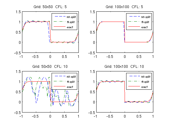
From the figure, we clearly see that highly inaccurate solutions are produced for both methods unless we have a sufficent grid resolution and a sufficient number of time steps. We notice that the front-tracking method gives a more accurate resolution of the shock than the NT scheme.

% NHR: please check what happens when CFL = 2.5 in the example above for
% the front-tracking solution.

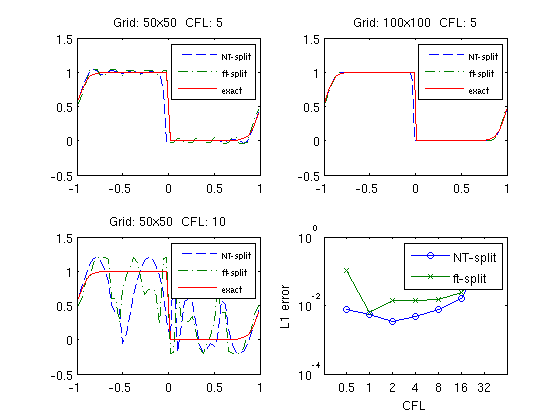
Effects of the CFL number.

Let us now investigate more closely the effects of varying CFL numbers

N     = 200;
delta = 1/sqrt(N);
h     = (xmax-xmin)/N;
x     = xmin:h:xmax;
y     = 0.5*(x(1:end-1)+x(2:end));
u0    = initialfunc(y,Kappa);

ft_err=zeros(1,7); cn_err=ft_err;
for k=1:7,
	CFL=2^(k-2);
	Nstep=ceil(T/(h*CFL));

	U=SourceSplit(u0,x,'burgerRsol','source',delta,Nstep,T,...
		'periodic',[xmin xmax],'wbar','kappa',Kappa,'fronttrack');
	ft_err(k)=h*sum(abs(U(Nstep+1,:)-U(1,:)));

	U=SourceSplit(u0,x,'burgerRsol','source',delta,Nstep,T,...
		'periodic',[xmin xmax],'wbar','kappa',Kappa,'central');
	cn_err(k)=h*sum(abs(U(Nstep+1,:)-U(1,:)));
end;
semilogy(-1:5,cn_err,'-o',-1:5,ft_err,'-x');
set(gca,'XTick',-1:5,'XTickLabel',2.^(-1:5));
xlabel('CFL'); ylabel('L1 error');
legend('NT-split','ft-split');

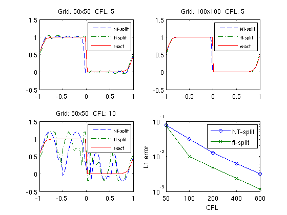
Grid refinement

Finally, we set the CFL number to 5 and conduct a grid-refinement study.

CFL=5;
ft_err = zeros(1,5); cn_err = ft_err;
for k=1:5,
	N     = 50*2^(k-1);
	delta = 1/sqrt(N);
   h     = (xmax-xmin)/N;
   x     = xmin:h:xmax;
   y     = 0.5*(x(1:end-1)+x(2:end));
   u0    = initialfunc(y,Kappa);

   Nstep=ceil(T/(h*CFL));
	U=SourceSplit(u0,x,'burgerRsol','source',delta,Nstep,T,...
		'periodic',[xmin xmax],'wbar','kappa',Kappa,'fronttrack');
	ft_err(k)=h*sum(abs(U(Nstep+1,:)-U(1,:)));

	U=SourceSplit(u0,x,'burgerRsol','source',delta,Nstep,T,...
		'periodic',[xmin xmax],'wbar','kappa',Kappa,'central');
	cn_err(k)=h*sum(abs(U(Nstep+1,:)-U(1,:)));
end;
semilogy(0:4,cn_err,'-o',0:4,ft_err,'-x');
set(gca,'XTick',0:4,'XTickLabel',50*2.^(0:4));
xlabel('CFL'); ylabel('L1 error');
legend('NT-split','ft-split');
ft_rate=log(ft_err(1:end-1)./ft_err(2:end))/log(2);
sft=strcat('Front track rate:',sprintf(' %3.2f',ft_rate));
cn_rate=log(cn_err(1:end-1)./cn_err(2:end))/log(2);
scn=strcat('Central rate    :',sprintf(' %3.2f',cn_rate));
disp(sft);
disp(scn);

Front track rate: 2.90 1.04 1.02 1.01
Central rate    : 1.34 1.29 1.01 1.00

rmpath ../Dimsplit/