Example 2.6: Balance Laws

In this example we will solve a scalar conservation law with a source

$$u_t + f(u)_x = g(u), \qquad u(x,0)=u_0(x)$

numerically by operator splitting. To this end, we use two substeps,

$S(t): \quad v_t + f(v)_x = 0, \qquad v(x,0)=v_0(x)$

$G(t): \quad w_t = g(w), \qquad w(y,0)=w_0(y)$

and construct the approximate solution from the formula

$u(x,t)\approx [G(\Delta t)\circ S(\Delta t) ]^n u_0(x)$

The hyperbolic step will be solved using the Lax-Friedrichs scheme and the ODE will be solved using MATLAB's ode45, which is a standard Runge-Kutta solver for nonstiff ODEs.

Initial setup

T  = 12;
N  = 512;
h  = 2*pi/N;
x  = -pi+(0:N)*h; x=0.5*(x(1:end-1)+x(2:end));
u0 = exp(-4*sin((x+2)/2).^2);
h  = path; path(h,'../Example2_5');

Burgers' equation with nonlinear source

As a concrete example we will use Burgers' equation with a nonlinear source term

$$ u_t + ( 0.5 u^2)_x = -u(1-u)(0.5-u) + 0.25 u$$

and periodic boundary conditions.

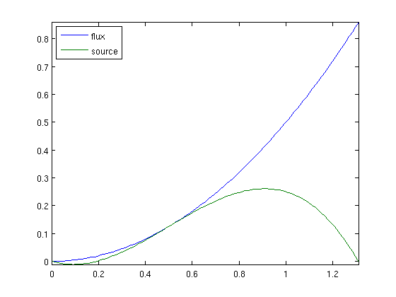
First, we plot the flux function and the nonlinear source function

u = linspace(0,1.31,101);
plot(u, flux(u), u, source(0,u)), axis tight, legend('flux','source',2)

Evolution of the shock profile

nsplit = 200;
u = sourcesplit('flux', 'source', u0, x, T, nsplit);
subplot(2,1,1), contourf(x,linspace(0,T,nsplit+1),u',20), colorbar
subplot(2,1,2), surf(x,linspace(0,T,nsplit+1),u')
shading interp; view(-10,50), axis tight

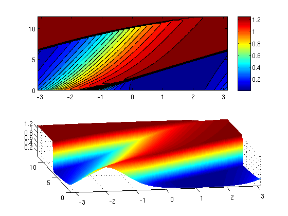
The initial smooth profile starts to travel to the right and sharpens up into a travelling shock wave followed by a rarefaction. Because of the nonlinear shape of the source term, we have negative accumulation in front of the shock (where u<0.2) and positive accumulation in the rarefaction (where u>0.2). Around t=6.5, the shock leaves the domain at the right-hand side and re-enters it at the left-hand side. The shock front then overtakes the rarefaction wave and the solution converges to the stationary solution u=1.3090..

Compare different time steps

Having established the dynamics of the problem, we can investigate the performance of our numerical method for different choices of the splitting step.

for n=1:4,
	nsplit = 8*4.^(n-1);
	u = sourcesplit('flux','source',u0,x,T,nsplit);
	subplot(2,2,n);
	contourf(x,linspace(0,T,nsplit+1),u');
   xlabel('x'), ylabel('time'), colorbar
	title([num2str(nsplit) ' steps'])
end
path(h);

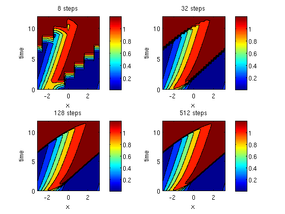
Even with only eight splitting steps, we are able to capture the major trends of the evolutionary behavior of our problem. However, to get rid of the artificial staircase behavior of the evoloving shock, we need to increase the number of splitting steps quite high.