Example 2.5: Viscous Conservation Law

In this example, we consider the viscous conservation law

$u_t + f(u)_x = \mu u_{xx}, \qquad u(x,0)=u_0(x).$

A common method to derive efficient methods for this equation is to split the evolution into two different operators

$S(t): \quad v_t + f(v)_x = 0, \qquad v(x,0)=v_0(x)$

$H(t): \quad w_t = \mu w_{xx}, \qquad w(y,0)=w_0(y)$

The approximate solution is constructed from the formula

$u(x,t)\approx [H(\Delta t)\circ S(\Delta t) ]^n u_0(x)$

This way, one can utilize highly efficient solvers for each of the two subequations. Here, we use a spectral difference method for the heat equation. Moreover, because the purpose here is simply to demonstrate the operator splitting, we use the simple first-order Lax-Friedrichs scheme for the hyperbolic conservation law ( $r=\Delta t/\Delta x$ )

$u_i^{n+1} = \frac12\bigl(u_{i-1}^n + u_{i+1}^n\bigr) - \frac12 r \bigl[ f(u_{i+1}^n) - f(u_{i-1}^n)\bigr]$

Initial setup

N  = 512; h = 2*pi/N;
T  = 6;
x  = -pi+(0:N)*h; x = 0.5*(x(1:end-1)+x(2:end));
u0 = exp(-4*sin((x+2)/2).^2);

Burgers' equation

A classical example of a viscous conservation law is the so-called Burgers' equation

$$ u_t + ( 0.5 u^2)_x = \mu u_{xx}

which can be considered a simplified model of the momentum equation from the Navier-Stokes equations. Here, we will consider the evolution of a smooth profile for \mu=0.01 using periodic boundary conditions.

nsplit = 50;
u = consheat('flux', u0, x, T, nsplit, 0.01);
subplot(2,1,1), plot(x,u(:,1:10:nsplit+1))
subplot(2,1,2), surf(x,linspace(0,T,nsplit+1),u')
shading interp; view(-10,50), axis tight

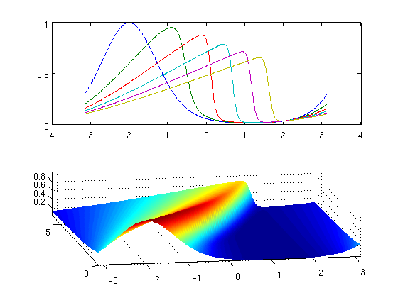
As we see from the figure, the nonlinear convective forces sharpen the smooth profile into a shock layer whose width is determined by the balance of the diffusion term and the self-sharpening mechanisms in the nonlinear flux function.

Compare different time steps

Next, we increase \mu to 0.1 and consider the effect of different number of splitting steps.

for n=1:4,
	nsplit = 4*3.^(n-1);
	u = consheat('flux', u0, x, T, nsplit);
   subplot(2,2,n); contourf(x, linspace(0,T,nsplit+1), u');
   xlabel('x'), ylabel('t'), colorbar, title([num2str(nsplit) ' steps']);
end;

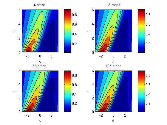
The approximations computed with four and twelve splitting steps clearly capture the dominant evolutionary behavior of the solution, but also contain nonphysical wiggles caused by splitting errors. As we increase the number of splitting steps, the splitting errors decrease and the approximate solutions are able to capture the whole evolution without significant artifacts created by our splitting strategy.

Comparing different shock widths

As a last example, we will look at the evolution of the smooth profile for different balances between the convective and diffusive forces.

mu = 4; nsplit = 50;
t  = linspace(0,T,nsplit+1);
for n=1:4,
   mu = 0.25*mu;
	u  = consheat('flux',u0,x,T,nsplit,mu);
	subplot(2,2,n); contourf(x,t,u');
   xlabel('x'), ylabel('t'), colorbar, title(['mu = ', num2str(mu)]);
end;

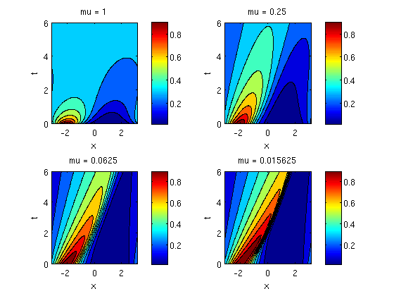
For large values of \mu, the diffusive forces dominate and the solution profile evolves toward a flat surface. As \mu decreases, the convective forces take over and the solution develops into a viscous shock that travels to the right.