2D Riemann Problem: Dimensional Splitting with Front Tracking

In this example, we consider the 2D scalar conservation law

$$ u_t + (u^2)_x/2 + (u^2)_y/2 = 0$$

with Riemann initial data, that is, with an intial function that has a constant value in each of the four quadrants and discontinuities along the x- and y-axes.

To solve the one-dimensional problems arising as part of the operator splitting, we will use front tracking followed by a projection step onto underlying regular grid.

Initial setup

N = 100;
h = 2/N;
x = -1:h:1;
y = 0.5*(x(1:end-1)+x(2:end));
T = 1.0;
delta = 0.1/sqrt(N);
[X,Y]=meshgrid(y,y);

Exact solutions

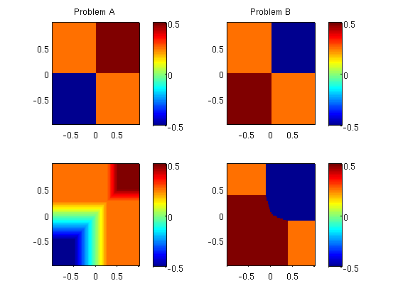
We consider two different setups. In both setups u0=1/4 in the second and fourth quadrant. Setting u0=1/2 in the first quadrant and u0=-1/2 in the third quadrant gives a self-similar wave pattern where the four original constant states are separated by two pairs of rarefaction waves. For each pair, the two rarefaction waves meet in a sharp kink along the line y = x. Switching the values in the first and third quadrant gives a wave pattern that consists of the four constant states separated by six shocks forming two triple points at (3t/8,−t/8) and (−t/8, 3t/8).

subplot(2,2,1), pcolor(X,Y,rpsola(X,Y,0)), shading flat; colorbar, title('Problem A')
subplot(2,2,2), pcolor(X,Y,rpsolb(X,Y,0)), shading flat; colorbar, title('Problem B')
subplot(2,2,3), pcolor(X,Y,rpsola(X,Y,1)), shading flat; colorbar
subplot(2,2,4), pcolor(X,Y,rpsolb(X,Y,1)), shading flat; colorbar

Riemann problem B: shocks

First, we study the error for the second Riemann problem as a function of the number of operator splitting steps

u0     = rpsolb(X,Y,0);
utrue  = rpsolb(X,Y,1);
rel    = sum(sum(abs(utrue)));
for i=1:4,
  Nstep = 4^(i-1);
  u     = DimSplit(u0,x,x,'burgerRsol','burgerRsol',delta,Nstep,T,'wbar');
  feil  = sum(sum(abs(utrue-u)))/rel;

  subplot(2,2,i);
  pcolor(y,y,u), axis equal image;  colorbar, shading flat
  title(sprintf('Grid: %dx%d  Steps: %d', N, N, Nstep));
  xlabel(sprintf('L1 error: %4.2f %%', 100*feil));
  p=get(gca,'position'); p([3 4])=p([3 4])+0.03;
  set(gca,'position',p,'XTickLabel',[]);
end;

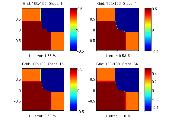
From the figure, we see that the error is a convex function of the number of splitting steps. With few splitting steps, the error is dominated by the splitting error and the strong self-sharpening effects present near the shocks will counteract the smearing introduced by the projection operator that brings the front tracking solution back from a possibly irregular grid and back to the underlying Cartesian grid. As the number of time steps increases, the number of projections increases and the self-sharpening effects of diminish so that the smearing errors become dominant. Because the two error mechanisms work in different directions, a minimum error is observed for an intermediate number of splitting steps.

Convergence test

We perform a grid-refinement study for the two Riemann problems, fixing the CFL number to 10 and report the error as a logarithmic plot

nu=10;
errA=ones(1,6); errB=errA;
for i=1:6,
  N     = 8*2^i;
  h     = 2/N;
  x     = -1:h:1;
  y     = 0.5*(x(1:end-1)+x(2:end));
  delta = 0.1/sqrt(N);
  [X,Y] = meshgrid(y,y);

  % Riemann problem A
  u       = DimSplit(rpsola(X,Y,0), x,x,'burgerRsol','burgerRsol', ...
                     delta, round(T/(nu*h)), T,'wbar');
  utrue   = rpsola(X,Y,1);
  rel     = sum(sum(abs(utrue)));
  errA(i) = sum(sum(abs(utrue-u)))/rel;

  % Riemann problem B
  u       = DimSplit(rpsolb(X,Y,0), x,x,'burgerRsol','burgerRsol', ...
                     delta, round(T/(nu*h)), T,'wbar');
  utrue   = rpsolb(X,Y,1);
  rel     = sum(sum(abs(utrue)));
  errB(i) = sum(sum(abs(utrue-u)))/rel;
end
clf, semilogy(4:9,errA,'-o',4:9,errB,'x-')
xlabel('log2 of grid size'); ylabel('Relative L1 error');
legend('Problem A','Problem B');

As pointed out above, the strong self-sharpening effects present near the shocks in Riemann problem B will counteract the smearing introduced by the projection operator leading to a convergence rate of approximately one. For the smooth solution resulting from Riemann problem A, the self-sharpening effects are much weaker, thereby giving a lower convergence rate.