Flow Past One, Two, and Three Cylinders
Front Tracking for the Euler Equations of Gas Dynamics
|
In this example we consider a Mach 3 flow past one, two, and three cylinders in a two dimensional domain [0,1]x[0,1]. Around the cylinders the density is initially 1.4 (equal the gas constant), the pressure is 1.0, and the velocities zero. The shock wave comes in from the left. All solutions are computed using front tracking and dimensional splitting on a 400x400 grid. At the cylinders we impose reflective boundaries, and the geometry is realized using a simple piecewise constant curve. The solutions suffer a bit from the poor approximation of the boundary. Furthermore, effects due to expansion shocks (for diffraction around corners) are also visible. Nevertheless, we feel that these examples demonstrates the ability of the method to handle quite complex geometries. |
|
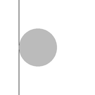
One CylinderThe cylinder has radius 0.2 and is placed at (0.4,0.5). To reach final computational time 0.16 we have used 160 time steps. Click on the link(s) below to see snapshots of the density depicted as Schlieren images. START the slide show.
[
t=0.00 |
t=0.02 |
t=0.04 |
t=0.06 |
t=0.08 |
t=0.10 |
t=0.12 |
t=0.14 ] |
|
Two CylindersThe cylinders have radius 0.1 and are placed at (0.30,0.30) and (0.35,0.70). To reach final computational time 0.16 we have used 160 time steps. Click on the link(s) below to see snapshots of the density depicted as Schlieren images. START the slide show.
[
t=0.00 |
t=0.02 |
t=0.04 |
t=0.06 |
t=0.08 |
t=0.10 |
t=0.12 |
t=0.14 |
t=0.16 ] |

|
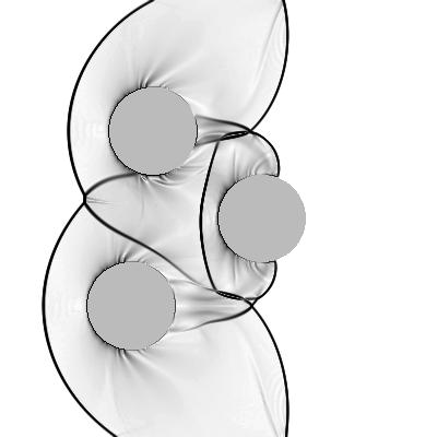
Three CylindersThe cylinders have radius 0.1 and are placed at (0.30,0.30), (0.35,0.70), and (0.60,0.50). To reach final computational time 0.25 we have used 250 time steps. Click on the link(s) below to see snapshots of the density depicted as Schlieren images. START the slide show.
[
t=0.000 |
t=0.025 |
t=0.050 |
t=0.075 |
t=0.100 |
t=0.125 ] |

|
Knut-Andreas Lie <andreas@math.ntnu.no> Last modified: Fri Jan 25 11:16:04 MET 2002